패턴명칭
Builder
필요한 상황
어떤 과정 거쳐 하나의 객체를 생성하는데, 그 과정에 대한 종류가 하나가 아닌 여러 개일때 사용할 수 있는 패턴이다.
예제 코드
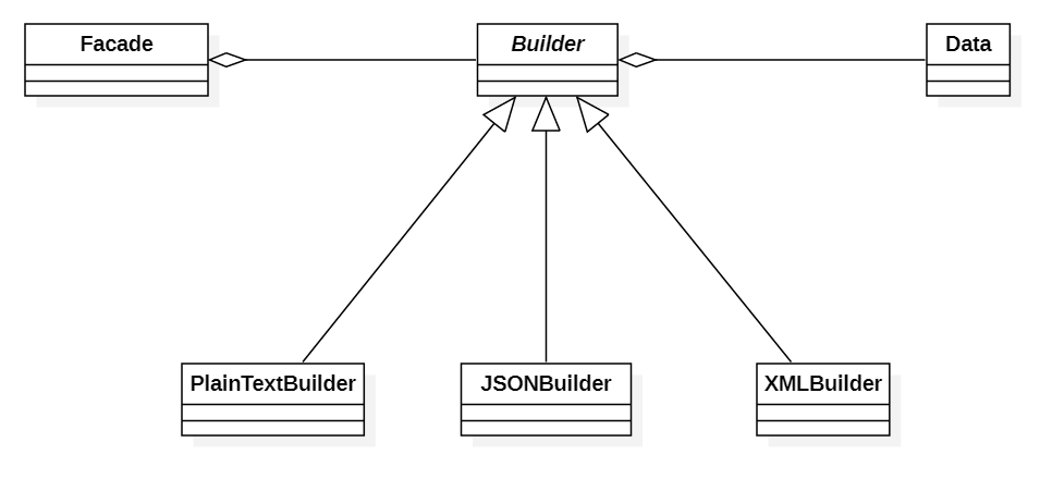
Data 클래스는 이름과 나이에 대한 데이터를 담고 있다. 이 Data 클래스에 대한 객체를 필요에 따라 평문 문자열 포맷이나 JSON 포맷 또는 XML 포맷의 문자열로 구성한다. 먼저 Data 클래스는 다음과 같다.
package pattern;

public class Data {
	private String name;
	private int age;

	public Data(String name, int age) {
		this.name = name;
		this.age = age;
	}

	public String getName() {
		return name;
	}

	public int getAge() {
		return age;
	}
}
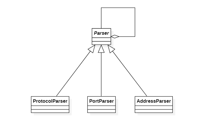
Builder 추상 클래스는 위의 Data를 다양한 포맷으로 구성하기 위한 공통된 인터페이스를 제공하는 부모 클래스이며 다음과 같다.
package pattern;

public abstract class Builder {
	protected Data data;

	public Builder(Data data) {
		this.data = data;
	}

	public abstract String head();
	public abstract String body();
	public abstract String foot();
}
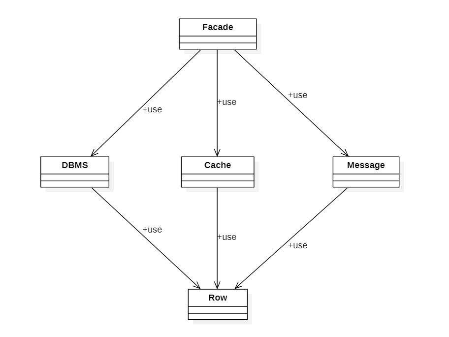
위의 Builder 클래스는 Facade 클래스에서 사용되는데, Facade 클래스는 다음과 같다.
package pattern;

public class Facade {
	private Builder builder;

	public Facade(Builder builder) {
		this.builder = builder;
	}

	public String build() {
		StringBuilder sb = new StringBuilder();

		sb.append(builder.head());
		sb.append(builder.body());
		sb.append(builder.foot());

		return sb.toString();
	}
}
Builder 클래스를 구현하는 파생 클래스를 보자. 먼저 평문 문자열 포맷으로 문자열을 구성하는 클래스인 PlainTextBuilder는 다음과 같다.
package pattern;

public class PlainTextBuilder extends Builder {
	public PlainTextBuilder(Data data) {
		super(data);
	}

	@Override
	public String head() {
		return "";
	}

	@Override
	public String body() {
		StringBuilder sb = new StringBuilder();

		sb.append("Name: ");
		sb.append(data.getName());
		sb.append(", Age: ");
		sb.append(data.getAge());

		return sb.toString();
	}

	@Override
	public String foot() {
		return "";
	}
}
다음은 JSON 포맷으로 구성하는 JSONBuilder 클래스이다.
package pattern;

public class JSONBuilder extends Builder {

	public JSONBuilder(Data data) {
		super(data);
	}

	@Override
	public String head() {
		return "{ ";
	}

	@Override
	public String body() {
		StringBuilder sb = new StringBuilder();

		sb.append("\"Name\": ");
		sb.append("\"" + data.getName() + "\"");
		sb.append(", \"Age\": ");
		sb.append(data.getAge());

		return sb.toString();
	}

	@Override
	public String foot() {
		return " }";
	}
}
다음은 XML 포맷으로 구성하는 XMLBuilder 클래스이다.
package pattern;

public class XMLBuilder extends Builder {

	public XMLBuilder(Data data) {
		super(data);
	}

	@Override
	public String head() {
		StringBuilder sb = new StringBuilder();

		sb.append("<?xml version=\"1.0\" encoding=\"utf-8\"?>");
		sb.append("<DATA>");

		return sb.toString();
	}

	@Override
	public String body() {
		StringBuilder sb = new StringBuilder();

		sb.append("<NAME>");
		sb.append(data.getName());
		sb.append("</NAME>");
		sb.append("<AGE>");
		sb.append(data.getAge());
		sb.append("</AGE>");

		return sb.toString();
	}

	@Override
	public String foot() {
		return "</DATA>";
	}
}
지금까지의 클래스를 사용하는 예제 코드는 다음과 같다.
package pattern;

public class Main {
	public static void main(String[] args) {
		Data data = new Data("Jane", 25);

		Builder builder = new PlainTextBuilder(data);
		Facade facade = new Facade(builder);
		String result = facade.build();
		System.out.println(result);

		builder = new JSONBuilder(data);
		facade = new Facade(builder);
		result = facade.build();
		System.out.println(result);

		builder = new XMLBuilder(data);
		facade = new Facade(builder);
		result = facade.build();
		System.out.println(result);
	}
}
실행결과는 다음과 같다.
Name: Jane, Age: 25
{ "Name" :"Jane", "Age": 25 }
<?xml version="1.0" encoding="utf-8"?><DATA><NAME>Jane</NAME><AGE>25</AGE></DATA>
이 글은 소프트웨어 설계의 기반이 되는 GoF의 디자인패턴에 대한 강의자료입니다. 완전한 실습을 위해 이 글에서 소개하는 클래스 다이어그램과 예제 코드는 완전하게 실행되도록 제공되지만, 상대적으로 예제 코드와 관련된 설명이 함축적으로 제공되고 있습니다. 이 글에 대해 궁금한 점이 있으면 댓글을 통해 남겨주시기 바랍니다.